Building an Image Classifier Using Keras

Machine Learning (ML) is disruptive technology that has taken the world by storm. It is the process where a computer learns to make predictions after observing some given data. It is used in Computer Vision, Natural Language Processing and Stock Price Prediction to name a few. The domain of ML is vast and it’s only going to get bigger. To demonstrate one such use of this technology, this article will talk about classifying pictures of the Avengers (namely Black Widow, Iron Man, Captain America, Hulk and Thor).

Image Source : Google

To begin with, we must collect some data for our model. For this we will scrape images from the internet. We will use the bing-image-downloader scraper tool. To install it, use the following command (all code written in Python 3) :

pip install bing-image-downloader

Then import the library:

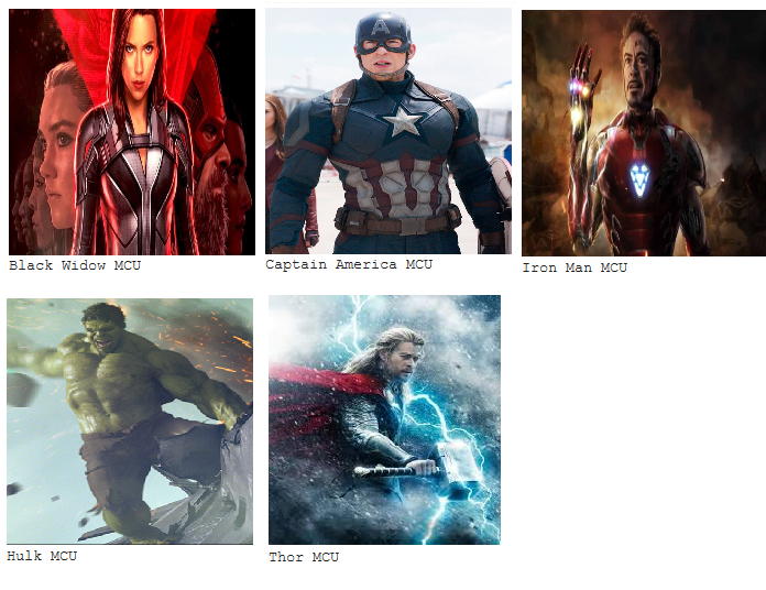
from bing_image_downloader import downloader

We have five classes in our data, namely, Black Widow, Iron Man, Captain America, Hulk and Thor. We will download 200 images of each class.

downloader.download('Iron Man MCU', limit = 200, output = 'datasets/Marvel Heroes/train', adult_filter_off = False, force_replace = False, timeout = 60)

We can follow the above code and replace the hero names to get different images.

Now that we have our images, we will split our images into three set : train (85 % of the data), validation (10 % of the data) and test (5 % of the data).

train_dir = 'datasets/Marvel Heroes/train/'
validation_dir = 'datasets/Marvel Heroes/validation/'
test_dir = 'datasets/Marvel Heroes/test/'

The train set will be used to train our data and the validation set will be used as guide measure our model’s performance during training. Finally, we’ll feed unseen images i.e. the test set and see how our model performs. The downloaded images are stored in the .jpg format and follows the name convention image_<number>.jpg. We create the respective directories as follows:

import os
import random #for splitting the data randomly
classes = os.listdir('datasets/Marvel Heroes/train/')
for hero in classes:
   j=0
   for i in random.randint(0,200):
       os.replace(train_dir + 'image_' + i + '.jpg', validation_dir + 'image_' + i + '.jpg')
       j=j+1
       if(j==20): #10 % of the images
          break
for hero in classes:
   j=0
   for i in random.randint(0,200):
       os.replace(train_dir + 'image_' + i + '.jpg', test_dir + 'image_' + i + '.jpg')
       j=j+1
       if(j==10): #5 % of the images
          break

After this step, we will begin modelling on our data. To save time, we’ll use a technique called Transfer Learning. It’s technique where we leverage the learning of a pre-trained Machine Learning model and use it for our purposes. It’s a common technique in the field of Computer Vision. We will use Keras on top of Tensorflow to accomplish this task. Keras is a beautiful API used a lot in the Machine Learning Community. The pre-trained model we will use is ResNet50.

from tensorflow.keras.layers import Dense
from tensorflow.keras.models import Sequential
from tensorflow.keras.applications.resnet50 import preprocess_input
from tensorflow.keras.applications import RestNet50

Let’s create our Model:

num_classes = 5
model = Sequential()
model.add(ResNet50(include_top = False, pooling='avg', weights = 'imagenet'))
model.add(Dense(num_classes, activation = 'softmax'))
model.layers[0].trainable=False 
#Don't train the top layer as this is we where will add our own classes 

We can have a look at our model parameters.

model.summary()

It will give the following output:

Model: "sequential_1"
_________________________________________________________________
Layer (type)                 Output Shape              Param #   
=================================================================
resnet50 (Functional)        (None, 2048)              23587712  
_________________________________________________________________
dense (Dense)                (None, 5)                 10245     
=================================================================
Total params: 23,597,957
Trainable params: 10,245
Non-trainable params: 23,587,712
_________________________________________________________________

We will now compile our model using the Adam Optimizer and calculate loss using Categorical Crossentropy and use the accuracy metric.

model.compile(optimizer='adam',loss='categorical_crossentropy',metrics=['accuracy'])

We’re done creating our model. Now we must feed the model data. For this, we will use the ImageDataGenerator which will also help us augment our data (adding noise like horizontal flips and rotation to the images).

from tensorflow.keras.preprocessing.image import ImageDataGenerator
train_datagen = ImageDataGenerator(preprocessing_function = preprocess_input, horizontal_flip = True, width_shift_range = 0.2 ,height_shift_range = 0.2)
)
val_datagen=ImageDataGenerator(preprocessing_function = preprocess_input)
train_generator = train_datagen.flow_from_directory(train_dir, target_size=(224,224), batch_size=32, class_mode='categorical')
validation_generator = val_datagen.flow_from_directory( validation_dir, target_size=(224,224), batch_size=5, class_mode='categorical')

It will generate the following output:

Found 850 images belonging to 5 classes.
Found 100 images belonging to 5 classes.

Let’s fit model.

history = model.fit(train_generator, epochs = 5, validation_data = validation_generator, verbose = 1)

The model will generate output similar to the following (may not be the same):

Epoch 1/5
25/25 [==============================] - 322s 13s/step - loss: 1.7210 - accuracy: 0.3485 - val_loss: 0.7263 - val_accuracy: 0.7222
Epoch 2/5
25/25 [==============================] - 185s 7s/step - loss: 0.6220 - accuracy: 0.7889 - val_loss: 0.5590 - val_accuracy: 0.8000
Epoch 3/5
25/25 [==============================] - 177s 7s/step - loss: 0.4306 - accuracy: 0.8484 - val_loss: 0.4328 - val_accuracy: 0.8556
Epoch 4/5
25/25 [==============================] - 172s 7s/step - loss: 0.2794 - accuracy: 0.9271 - val_loss: 0.3850 - val_accuracy: 0.8667
Epoch 5/5
25/25 [==============================] - 167s 7s/step - loss: 0.2736 - accuracy: 0.9281 - val_loss: 0.3570 - val_accuracy: 0.8778

Voila! Looks like we got ~88 % accuracy on the validation set and ~93 % on the train set. Not Bad! Let’s plot our results.

import matplotlib.pyplot as plt
acc = history.history['accuracy']
val_acc = history.history['val_accuracy']
loss = history.history['loss']
val_loss = history.history['val_loss']
epochs = range(len(acc))
plt.plot(epochs, acc)
plt.plot(epochs, val_acc)
plt.title('Training and validation accuracy')
plt.legend(['Train','Val'])
plt.figure() #Train accuracy
plt.plot(epochs, loss)
plt.plot(epochs, val_loss)
plt.title('Training and validation loss')
plt.legend(['Train','Val']) #Train Loss

It will generate the following plots:

Plots

We can save the model as follows:

model.save('/Created Models/')

Let’s do some predictions now. Import the following libraries.

from keras.preprocessing.image import load_img
from keras.preprocessing.image import img_to_array
from keras.preprocessing.image import array_to_img

Now for predictions.

for im in os.listdir(test_dir):
      image = load_img(os.path.join(test_dir,im),target_size=(224,224))
      input_arr = img_to_array(image)
      input_arr = np.expand_dims(input_arr,axis=0)
      input_arr = preprocess_input(input_arr)
      pred = model.predict(input_arr)
      maxPosition = np.argmax(pred)
      pred_label = classes[maxPosition]
      display(image)
      print(pred_label)
      print()
      print()

Some of the predictions are as follows:

Some of the test set.

That’s the end of the article. Hope you enjoyed it. See you later!